Gaussian Processes are Not So Fancy

Wednesday December 26, 2018

Gaussian Processes have a mystique related to the dense probabilistic terminology that's already evident in their name. But Gaussian Processes are just models, and they're much more like k-nearest neighbors and linear regression than may at first be apparent.

Gaussian Processes have applications ranging from finding gold to optimizing hyperparameters of other models. The focus here is on how Gaussian Processes work, using an example that's simple enough to show completely from beginning to end.

A simple training data set

A model is trained with predictors \( X \) and known labels \( y \). Here's some data in Python:

train_X = [[0.8], [1.2], [3.8], [4.2]]
train_y = [   3,     4,    -2,    -2 ]

Since elements of \( X \) are one-dimensional, all the data can be shown in a simple figure:

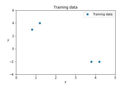
The task of a model is to predict \( y \) values for test points \( x \).

Applying a kernel function

Like SVMs, Gaussian Processes use kernel functions. A kernel gives a closeness, or similarity, between two points. This is related to distances, and a kernel may involve distance. Here's the matrix of Euclidean distances between points in our training data \( X \):

dist_XX = sklearn.metrics.pairwise_distances(train_X)
## array([[0. , 0.4, 3. , 3.4],
##        [0.4, 0. , 2.6, 3. ],
##        [3. , 2.6, 0. , 0.4],
##        [3.4, 3. , 0.4, 0. ]])
# Recall:
# train_X = [[0.8], [1.2], [3.8], [4.2]]

The Gaussian radial basis function (RBF) kernel is commonly used. In Gaussian Processes for Machine Learning, Rasmussen and Williams call it the squared exponential kernel, probably to avoid confusion with other things that are Gaussian. For distance \( d \), it's \( e^{-\frac{1}{2}d^2}\):

def squared_exponential(distance):
    return np.exp(distance**2 / -2)

It's one when distance is zero, and it goes to zero when distance is big. This is evident for our data when we make the matrix of kernel values for the training data \( X \):

kern_XX = squared_exponential(dist_XX)
## array([[1.  , 0.92, 0.01, 0.  ],
##        [0.92, 1.  , 0.03, 0.01],
##        [0.01, 0.03, 1.  , 0.92],
##        [0.  , 0.01, 0.92, 1.  ]])
# Recall:
# train_X = [[0.8], [1.2], [3.8], [4.2]]

This matrix \( K(X, X) \) is a core component of Gaussian Processes, and as the example shows, it reflects a core concern with nearness as represented via a kernel function.

Using the Gaussian Process prediction equation

This is Rasmussen and Williams' Equation 2.19 for the predictive posterior distribution, which I promise isn't as bad as it looks:

\[ \mathbf{f_{\ast}} | X_{\ast}, X, \mathbf{f} \sim \mathcal{N}( K(X_{\ast}, X) K(X,X)^{-1} \mathbf{f}, \\ K(X_{\ast}, X_{\ast}) - K(X_{\ast}, X) K(X,X)^{-1} K(X, X_{\ast}) ) \]

Here \( \mathbf{f_{\ast}} \) is the predicted \( y \) for a test point in \( X_{\ast} \) based on the training data \( X \) and \( y \) labels \( \mathbf{f} \). It's predicted to be normally distributed with mean \( K(X_{\ast}, X) K(X,X)^{-1} \mathbf{f} \) and the given covariance. The mean can be considered "the" prediction, though you can also sample.

Behaves like nearest neighbors

Let's use Equation 2.19 to make a prediction for this \( X_{\ast} \):

test_X = [[1]]

We find the kernel similarities between the test point and each point of training data:

kern_xX = squared_exponential(
              sklearn.metrics.pairwise_distances(test_X, train_X))
## array([[0.98019867, 0.98019867, 0.01984109, 0.00597602]])

The test point is close to the first two training points, and far from the second two.

Let's evaluate just the first two terms of the predictive mean given in Equation 2.19:

kern_xX.dot(np.linalg.inv(kern_XX))
## array([[ 0.50835358,  0.51127124, -0.01378216,  0.01144869]])

It isn't exactly, but this looks a lot like a weighting for a weighted average. And the prediction roughly fits that interpretation:

test_y = kern_xX.dot(np.linalg.inv(kern_XX)).dot(train_y)[0]
## 3.57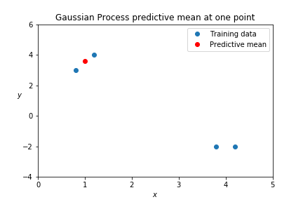

This behavior is similar to k-nearest neighbors. Nearby points matter; points that are far away don't. Nearest neighbors can even include a weighting based on a kernel function.

Also like k-nearest neighbors, you have to use the whole training set for every Gaussian Process prediction, comparing the test point to every training point.

With Gaussian Processes, however, you don't have to specify a number of neighbors \( k \). Every point that is near enough contributes to the prediction.

The comparison here to a kind of weighted average nearest neighbors is much more directly valid for kernel regression, which is another technique that also uses kernels. With Gaussian Processes, there's really a further step of curve-fitting going on.

It's linear regression

The mean prediction of a Gaussian Process is the same as a linear regression with a particular choice of coordinates. Let's talk about how.

Why is \( K(X,X)^{-1} \) involved in the predictive mean?

Consider the kernel matrix as a transformation of the original training data \( X \) into new variables, where each of the new variables is kernel-nearness to one of the points of training data. This is very much like transforming raw data to include interactions or polynomial terms, as is common in regression. Say the transformed data is \( Z \).

Linear regression coefficients can be solved for with \( (Z^T Z)^{-1} Z^T \). But with a nice symmetric square matrix like \( K(X,X) \), this is the same as just taking \( Z^{-1} \) directly.

So the mean prediction of a Gaussian Process is the same as linear regression in the coordinates defined by kernel similarities with each training point. It is linear regression.

With covariance

With Gaussian Processes, kernel functions are also called covariance functions. Things that are kernel-near vary together—they have similar values—and this enforces smoothness.

Here's the covariance part of Equation 2.19 again. It has two terms:

\[ K(X_{\ast}, X_{\ast}) - K(X_{\ast}, X) K(X,X)^{-1} K(X, X_{\ast}) \]

The positive first term shows that test point(s) vary together when they're close to one another. The negative second term (which is also a linear regression solution, like the mean) captures how much variance is eliminated due to being close to observed points.

Predicting for multiple points

If you get the predictive mean for many points, you can draw out a curve:

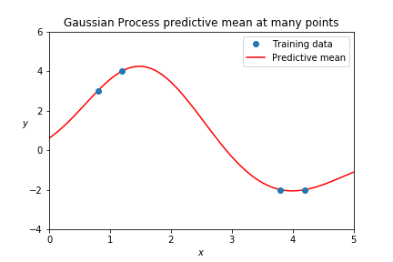
You may instead want to use the predictive mean and variance at some test point to sample an outcome \( y \). If you then take that sampled value as a new point of training data (adding it to your training set) future predictions will be consistent with that first one, and so on.

You can equivalently make multiple consistent predictions simultaneously by putting multiple test points in \( X_{\ast} \) and sampling from a multivariate Gaussian.

Just like the mean alone, values sampled this way will draw out a smooth curve. But unlike the mean alone, each random draw will be a different curve: Gaussian Processes are random over a space of functions. An approachable post by Bailey focuses on this.

It can be fun to sample curves, but often the mean and variance alone are useful.

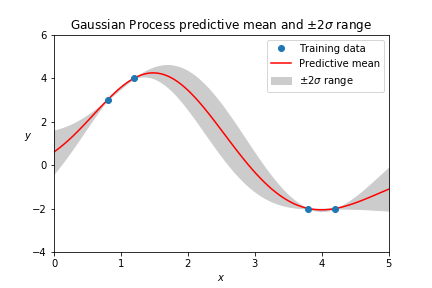
The Bayesian prior away from data

Gaussian Processes have Bayesian priors. For the example here, the assumption is that the function is always zero with covariance one, until we see training data showing otherwise.

In Equation 2.19, you can think of the mean as zero plus contributions from the training data; that's where the zero comes from. Covariance comes from the kernel function, which gets as big as one. To change the prior on the covariance, change the kernel function.

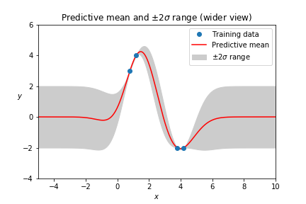
The prior is visible when the bounds of the plot are expanded, which illustrates that Gaussian Processes often focus on local interpolation more than extrapolation.

Length scale matters

The kernel specifies the scale of the variance, and in the case of the squared exponential kernel, there's also a length scale parameter that has significant effects.

def squared_exponential(distance, length_scale=1):
    return np.exp((distance / length_scale)**2 / -2)

For our example, a length scale of one works reasonably well. For a smaller length scale, the function is allowed to change faster, and the prior asserts itself more quickly:

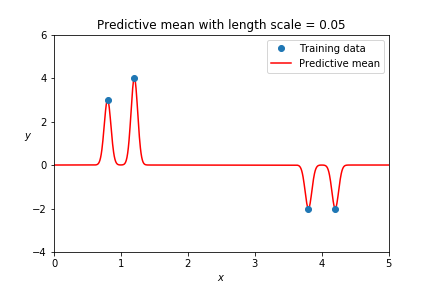
For a Gaussian Process to capture a trend, its kernel needs to support it. In the case of the squared exponential kernel, this means a long enough length scale.

When hyperparameters are your parameters

As presented here, a Gaussian Process will always exactly fit its training data. This is often considered a sign of overfitting, and regardless it's clearly unsustainable if training data ever has two different \( y \) values for identical \( x \) values.

Noise can be added to address these issues, and the scale of the noise is another hyperparameter, joining the overall scale and length scale of the covariance function.

To get really interesting behavior may require composing kernel functions, altering what "near" means for the model and adding even more hyperparameters, as in this example.

Gaussian Process implementations like sci-kit's try to automatically fit these hyperparameters, which may remove some of the need to know what they should be in advance. But optimization can't do all the work of designing an appropriate kernel for a problem, or eliminate the difficulty of distances in high-dimensional spaces.

There are also some approaches for improving computational efficiency.

Not useless, but not magical

Even with enhancements, the fundamental nature of Gaussian Processes is as presented here: local smooth curve fitting built on linear regression.

A Gaussian Process might be useful for you. But please don't assume that it is sophisticated just because the language around it often is, or that its results are automatically true just because they have error bars.

The code and plots from this post are all in a Jupyter notebook.

Thanks to Erica Blom, Marco Pariguana, Sylvia Blom, Travis Hoppe, and Ajay Deonarine for reading drafts of this post and providing feedback. Thanks also to everybody on Reddit, on HN, on DataTau, on Twitter, on Pinboard, and elsewhere!