See sklearn trees with D3
Sunday November 29, 2015
The decision trees from scikit-learn are very easy to train and predict with, but it's not easy to see the rules they learn. The code below makes it easier to see inside sklearn classification trees, enabling visualizations that look like this:
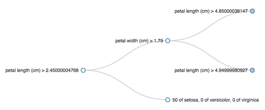
This shows, for example, that all the irises with petal length (cm) less than 2.45 were setosa.
The ability to interpret the rules of a decision tree is often considered a strength of the algorithm, and in R you can usually summary() and plot() a tree fit to see the rules. In Python with sklearn, there is export_graphviz, but it isn't terribly convenient. It shouldn't be so hard to see what's going on inside a tree.
The following JSON format is simple and works with common D3 tree graphing code, so let's target this format:
{name: "container thing",
 children: [{name: "leaf thing one"},
            {name: "leaf thing two"}]}
Each name will describe a true/false decision rule for an inner node or the distribution of training example labels for a leaf node. The first of a pair of children is where the rule is true, and the second is where the rule is false. (These are binary trees.)
The way sklearn trees store their rules internally is described in _tree.pyc. The rules function here examines a fit sklearn decision tree to generate a Python dictionary (with structure like the above) representing the decision tree's rules:
def rules(clf, features, labels, node_index=0):
    """Structure of rules in a fit decision tree classifier

    Parameters
    ----------
    clf : DecisionTreeClassifier
        A tree that has already been fit.

    features, labels : lists of str
        The names of the features and labels, respectively.

    """
    node = {}
    if clf.tree_.children_left[node_index] == -1:  # indicates leaf
        count_labels = zip(clf.tree_.value[node_index, 0], labels)
        node['name'] = ', '.join(('{} of {}'.format(int(count), label)
                                  for count, label in count_labels))
    else:
        feature = features[clf.tree_.feature[node_index]]
        threshold = clf.tree_.threshold[node_index]
        node['name'] = '{} > {}'.format(feature, threshold)
        left_index = clf.tree_.children_left[node_index]
        right_index = clf.tree_.children_right[node_index]
        node['children'] = [rules(clf, features, labels, right_index),
                            rules(clf, features, labels, left_index)]
    return node
How is this used? Let's get a quick example decision tree and take a look:
from sklearn.datasets import load_iris
from sklearn.tree import DecisionTreeClassifier

data = load_iris()

clf = DecisionTreeClassifier(max_depth=3)
clf.fit(data.data, data.target)

rules(clf, data.feature_names, data.target_names)
The rules function returns the following Python dictionary, formatted for readability here:
{'name': 'petal length (cm) > 2.45000004768',
 'children': [
     {'name': 'petal width (cm) > 1.75',
      'children': [
         {'name': 'petal length (cm) > 4.85000038147',
          'children': [
              {'name': '0 of setosa, 0 of versicolor, 43 of virginica'},
              {'name': '0 of setosa, 1 of versicolor, 2 of virginica'}]},
         {'name': 'petal length (cm) > 4.94999980927',
          'children': [
              {'name': '0 of setosa, 2 of versicolor, 4 of virginica'},
              {'name': '0 of setosa, 47 of versicolor, 1 of virginica'}]}]},
     {'name': '50 of setosa, 0 of versicolor, 0 of virginica'}]}
This is pretty readable, but now we can also write the result out to a file and visualize it with D3:
import json

r = rules(clf, data.feature_names, data.target_names)
with open('rules.json', 'w') as f:
    f.write(json.dumps(r))
Check out the interactive view! Once again, a partially expanded view looks like this: