Practical Mergic
Wednesday May 20, 2015
A talk for the New York Open Statistical Programming Meetup on Wednesday May 20, 2015. Including some material originally given in a lightning talk at the May meeting (registration) of the PyData NYC meetup group.
@planarrowspace
Hi! I'm Aaron. This is my blog and my twitter handle. You can get from one to the other. This presentation and a corresponding write-up (you're reading it) are on my blog (which you're on).

The first time I wrote software to address this problem, I was working for the New York City Department of Education, in Tweed Courthouse.
The NYC DOE had unique IDs for every student, and for every teacher, but did not have unique IDs for principals. This was the case at least for some of the data system at that time. And this made sense, because there are only about sixteen hundred New York City public schools.
Those of you who have experience with humans will know that names are not unique IDs. People change their names, or add titles like “PhD”, or have their names entered differently at different times for no good reason. In the case of principals, sometimes they switch schools and change their names at the same time.
The DOE makes some decisions based on data, God bless them. The data associated with a principal might determine whether they get a bonus or an unpleasant phone call. In a situation like this, an approximate matching solution is not acceptable.
I had to get a perfect matching of all these principals' names, so I wrote some code to help speed the process. I had to verify the match by pairs, and it was awful, and I wished there was a better way to do it.
My primary concerns were, and are, to speed up the de-duplication process while allowing corrections by hand—still being reproducible and easily auditable by humans.
Since then, I've developed a process, or workflow, that I think is pretty good, and I've written a new tool to help with this process.
I've also learned about some of the broader ecosystem of techniques and tools available, and I'll talk about these as well.
I'll finish by suggesting that we probably need to do something entirely different. I'd like to encourage a discussion that could lead to more and better work with data.
“There are only two hard things in computer science: cache invalidation and naming things.”
Phil Karlton said that “There are only two hard things in computer science: cache invalidation and naming things.”
When working with data (let's call it “data science” then, instead of “computer science”) you have problems not only with your own names, but also with everybody else's names.
It's just semantics, I suppose.
What are we talking about?
이름이란 것은 정말 중요합니다. 예를 들면, 미국에서 한국말로...
My Korean isn't that good. What I'm trying to say here is that agreeing on names is important, and the issue is a big one.
Maintaining a practical focus, let's look at just two classes of problems:
when names are the same
Lots of things can go wrong when names are re-used when they shouldn't be.
when names aren't the same
It can be even worse when names for the same thing are not the same.
Both these problems are closely related to merging, and we'll think a lot about that context.
But first, an example illustrating the importance of checking that your names are unique (that is, not ever the same).
demo: DOE data
The Excel file here was downloaded from the NYC DOE site. It contains standardized test results for New York City schools for individual grades and other sub-groups. We'll use two sheets that have been saved as CSV (originally for my Clean Data with R talk), gender.csv and all.csv. The R script itself is in check_unique.R.
There's a little setup to make reading in the data easier.
library("dplyr")

read.doe <- function(filename) {
  data <- read.csv(filename, as.is=TRUE,
                   skip=6, check.names=FALSE,
                   na.strings="s")
  stopifnot(names(data) == c("DBN", "Grade", "Year", "Category",
                             "Number Tested","Mean Scale Score",
                             "#","%","#","%","#","%","#","%","#","%"))
  names(data) <- c("dbn", "grade", "year", "category",
                   "num_tested", "mean_score",
                   "num1", "per1", "num2", "per2", "num3", "per3",
                   "num4", "per4", "num34", "per34")
 return(tbl_df(data))
}
Now we can start looking at the data, using dplyr:
gender <- read.doe("gender.csv")

gender
## Source: local data frame [68,028 x 16]
##
##       dbn grade year category num_tested mean_score num1 per1 num2 per2
## 1  01M015     3 2006   Female         23        675    0  0.0    7 30.4
## 2  01M015     3 2006     Male         16        657    2 12.5    4 25.0
## 3  01M015     3 2007   Female         11        679    2 18.2    0  0.0
## 4  01M015     3 2007     Male         20        668    0  0.0    3 15.0
## 5  01M015     3 2008   Female         17        661    0  0.0    5 29.4
## 6  01M015     3 2008     Male         20        674    0  0.0    1  5.0
## 7  01M015     3 2009   Female         13        667    0  0.0    1  7.7
## 8  01M015     3 2009     Male         20        668    0  0.0    3 15.0
## 9  01M015     3 2010   Female         13        681    2 15.4    7 53.8
## 10 01M015     3 2010     Male         13        673    4 30.8    5 38.5
## ..    ...   ...  ...      ...        ...        ...  ...  ...  ...  ...
## Variables not shown: num3 (int), per3 (dbl), num4 (int), per4 (dbl), num34
##   (int), per34 (dbl)
What's our unique key for this data set? It looks like it should be dbn (a unique identifier for a school), grade, year, and category. Let's check. The following should be zero if there are no duplicates.
gender %>%
  select(dbn, grade, year, category) %>%
  duplicated %>%
  sum
## [1] 1421
Shocking! Seeing that there are duplicates doesn't yet tell us how the duplicates are distributed; is it 1,422 copies of the same combination, or something else?
gender %>%
  group_by(dbn, grade, year, category) %>%
  summarize(n=n()) %>%
  group_by(n) %>%
  summarize(count=n())
## Source: local data frame [2 x 2]
##
##   n count
## 1 1 65186
## 2 2  1421
Much like using table, now we can see that most key combinations appear just once, but 1,421 appear twice. Interesting! Let's look at them.
gender %>%
  group_by(dbn, grade, year, category) %>%
  filter(1 < n())
## Source: local data frame [2,842 x 16]
## Groups: dbn, grade, year, category
##
##       dbn      grade year category num_tested mean_score num1 per1 num2
## 1  01M019          3 2010     Male         20        677    3   15    7
## 2  01M019          3 2010     Male          2         NA   NA   NA   NA
## 3  01M019          4 2010     Male         20        674    1    5    9
## 4  01M019          4 2010     Male          1         NA   NA   NA   NA
## 5  01M019          5 2010     Male          1         NA   NA   NA   NA
## 6  01M019          5 2010     Male         17        688    0    0    3
## 7  01M019 All Grades 2010     Male          4         NA   NA   NA   NA
## 8  01M019 All Grades 2010     Male         57         NA    4    7   19
## 9  01M020          3 2010     Male         50        686    8   16   15
## 10 01M020          3 2010     Male          1         NA   NA   NA   NA
## ..    ...        ...  ...      ...        ...        ...  ...  ...  ...
## Variables not shown: per2 (dbl), num3 (int), per3 (dbl), num4 (int), per4
##   (dbl), num34 (int), per34 (dbl)
Looks like there are two different kinds of males! How strange! Can we see what's going on by looking at the rest of the file?
gender %>%
  filter(dbn=='01M019', year==2010, grade==3)
## Source: local data frame [3 x 16]
##
##      dbn grade year category num_tested mean_score num1 per1 num2 per2
## 1 01M019     3 2010   Female         16        687    0    0    9 56.3
## 2 01M019     3 2010     Male         20        677    3   15    7 35.0
## 3 01M019     3 2010     Male          2         NA   NA   NA   NA   NA
## Variables not shown: num3 (int), per3 (dbl), num4 (int), per4 (dbl), num34
##   (int), per34 (dbl)
Unfortunately not; we'll have to look at additional data to try to determine what's going on. (This is typical.)
all_students <- read.doe("all.csv")
data <- bind_rows(all_students, gender)

data %>%
  filter(dbn=='01M019', year==2010, grade==3)
## Source: local data frame [4 x 16]
##
##      dbn grade year     category num_tested mean_score num1 per1 num2 per2
## 1 01M019     3 2010 All Students         36        682    3  8.3   16 44.4
## 2 01M019     3 2010       Female         16        687    0  0.0    9 56.3
## 3 01M019     3 2010         Male         20        677    3 15.0    7 35.0
## 4 01M019     3 2010         Male          2         NA   NA   NA   NA   NA
## Variables not shown: num3 (int), per3 (dbl), num4 (int), per4 (dbl), num34
##   (int), per34 (dbl)
It looks like these extra males aren't being counted in the total for “All Students”, so maybe we can drop them. Or maybe the “All Students” total is wrong.

Original image from Magnolia via Indie Outlook.
“This happens. This is a thing that happens.”
This is a scene from a movie called Magnolia when it's raining frogs. One of the things they say in that movie is that strange things happen, and if you've worked with any variety of data sets, you've probably encountered very strange things. You need to check everything—including things that you shouldn’t have to check.
(One good way to check is to use Tony's Assertive R package!)
merge
One big reason to want nice unique IDs is that you would like to merge two data sets, and you need something to match records by. Let's do a quick refresher on merging, or joining.
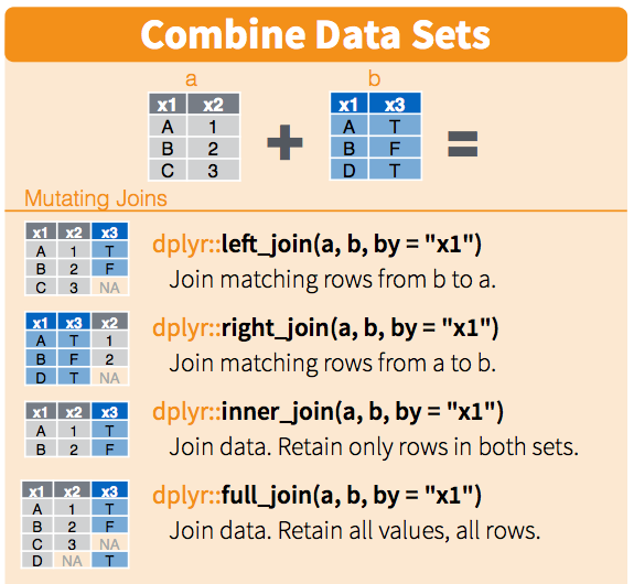
This is a section from RStudio's cheatsheet for dplyr. These cheatsheets are fantastic.
We'll do a merge between two data sets. For simplicity say that they have one column which is an identifier for each row, and some data in other columns. There are a couple ways we can join the data.
Some people like to think about these in terms of Venn diagrams.
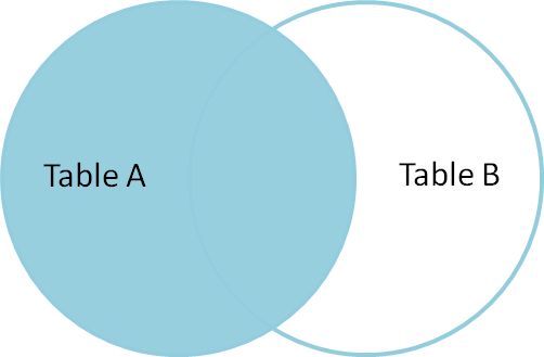
This picture comes from Jeff Atwood's post called visual explanation of SQL joins.
A former co-worker told me that seeing these pictures changed his life. I hope you like them.
This is a left join: you get all the keys from the left data set, regardless of whether they're in the right data set.
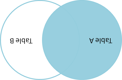
Jeff Atwood doesn't have a picture of a right join on his blog, but you can make one with a little ImageMagick.
$ convert -rotate 180 left_join.png right_join.pngYou're welcome.
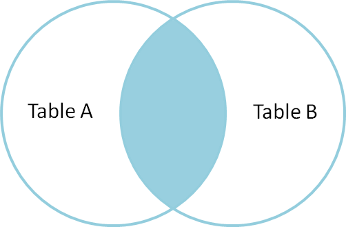
An inner join, or natural join, only gives you results for keys that appear in both the left and right data sets.

And an outer join gives you everything. Great!
There are a few other terms we could add, but let's not.

Here's the dplyr summary again. You can see how you can introduce missing values when doing left, right, and outer joins.
Ready? Here's a test.
How many rows do you get when you outer join two tables?
Think about this question, discuss it with somebody near you, come up with everything you can say about the number of rows you might expect when you join two tables. Introduce any quantities you think you'd like to know.
Take about three minutes and then come back.
three minutes pass
Say there are \( N \) rows in the first table and \( M \) rows in the second table. Then the smallest number of rows we can get from the outer join is the greater of \( N \) and \( M \). But we might get as many as \( N \cdot M \) rows, if all the keys are the same!
If you said the maximum was \( N + M \), you were probably assuming, implicitly or explicitly, that all they keys were unique. This is a common assumption that you should really check.
> nrow(first)
## [1] 3
> nrow(second)
## [1] 3
> result <- merge(first, second)
> nrow(result)
## [1] 3
This code is runnable in count_trouble.R.
Is it enough to check the numbers of rows when we do joins?
This does an inner join, which is the default for merge in R.
Think about it.
 x    y1        x   y2        x    y1   y2
 1 looks        1 good        1 looks good
 2    oh        2  boy        2    oh  boy
 3  well        2   no        2    oh   no
There is no peace while you don't have unique IDs.
There are times when you don't want every ID to be unique in a table, but really really often you do. You probably want to check that uniqueness explicitly.
when names are the same
This has been a discussion of problems arising from names being the same.
when names aren't the same
And now, you probably also want to check that the intersection you get is what you expect.
You don't want to silently drop a ton of rows when you merge!
This is the beginning of our problems with names that aren't the same.
demo: let's play tennis
Here begins material also present in ajschumacher/mergic:tennis.
Download the Tennis Major Tournament Match Statistics Data Set from the UC Irvine Machine Learning Repository into an empty directory:
$ wget https://archive.ics.uci.edu/ml/machine-learning-databases/00300/Tennis-Major-Tournaments-Match-Statistics.zipThis file should be stable, but it's also included here and/or you can verify that its md5 is e9238389e4de42ecf2daf425532ce230.
Unpack eight CSV files from the Tennis-Major-Tournaments-Match-Statistics.zip:
$ unzip Tennis-Major-Tournaments-Match-Statistics.zipYou should see that the first two columns of each file contain player names, though the column names are not consistent. For example:
$ head -2 AusOpen-women-2013.csv | cut -c 1-40
## Player1,Player2,Round,Result,FNL1,FNL2,F
## Serena Williams,Ashleigh Barty,1,1,2,0,5

$ head -2 USOpen-women-2013.csv | cut -c 1-40
## Player 1,Player 2,ROUND,Result,FNL.1,FNL
## S Williams,V Azarenka,7,1,2,1,57,44,43,2
Make a names.txt with all the names that appear:
$ for filename in *2013.csv
do
    for field in 1 2
    do
        tail +2 $filename | cut -d, -f$field >> names.txt
    done
done
Now you have a file with 1,886 lines, each one of 669 unique strings, as you can verify:
$ wc -l names.txt
## 1886

$ sort names.txt | uniq | wc -l
## 669
There are too many unique strings—sometimes more than one string for the same player. As a result, a count of the most common names will not accurately tell us who played the most in these 2013 tennis competitions.
$ sort names.txt | uniq -c | sort -nr | head
##  21 Rafael Nadal
##  17 Stanislas Wawrinka
##  17 Novak Djokovic
##  17 David Ferrer
##  15 Roger Federer
##  14 Tommy Robredo
##  13 Richard Gasquet
##  11 Victoria Azarenka
##  11 Tomas Berdych
##  11 Serena Williams
The list above is not the answer we’re looking for. We want to be correct.
single field deduplication
We're going to think about this problem, which is pretty common, of de-duplicating (or making a merge table for) a single text field.
Lukas Lacko             F Pennetta
Leonardo Mayer          S Williams
Marcos Baghdatis        C Wozniacki
Santiago Giraldo        E Bouchard
Juan Monaco             N.Djokovic
Dmitry Tursunov         S.Giraldo
Dudi Sela               Y-H.Lu
Fabio Fognini           T.Robredo
...                     ...
Here begins material also presented in a lightning talk at the May meeting (registration) of the PyData NYC meetup group.
To be clear, the problem looks like this. And the problem often looks like this: You have either two columns with slightly different versions of identifiers, or one long list of things that you need to resolve to common names. These problems are fundamentally the same.
Do you see the match here? (It's Santiago!)
So we need to find the strings that refer to the same person.
demo: Open Refine
Open Refine is quite good.
An interesting side story is that Open Refine was formerly Google Refine, and before that Metaweb's “Freebase Gridworks”. Google is shutting down Freebase, and we have to hope that Wikidata will then be the open match for Google's Knowledge Graph.
Thanks to Joel Natividad for pointing out an interesting algorithmic development connected with ongoing work on Open Refine. He also pointed out that there is a Python module called refine-client for using Open Refine from Python.
Steps of simple Open Refine demo:
- Start the Open Refine app
- Browse to http://localhost:3333/
- Click “Create Project”
- Click “Choose Files”
- Select
names.txt - Click “Next »“
- Click “Create Project »”
- Click the down arrow next to “Column 1”, then follow “Edit cells” to “Cluster and edit…”
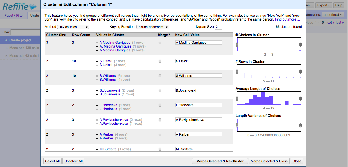
Open Refine has introductory and in-depth documentation about their “clustering” mechanisms.
In this interface, we can use “key collision” or “nearest neighbor” methods.
The “key collision” method maps every value to one “key”, and items are identical if they have the same key. This allows us to avoid calculating anything for all pairs. (This should remind you of hashing.)
There are four “keying functions” in Open Refine:
- “fingerprint” standardizes a string by case and punctuation.
- “ngram-fingerprint” standardizes a bit further, using character ngrams.
- “metaphone3” standardizes by the phonetic Metaphone 3 algorithm so that things that sound the same in English should be keyed together. (There are strange licensing issues around Metaphone 3.)
- “cologne-phonetic” standardizes by the Kölner Phonetik algorithm so that things that sound the same in German should be keyed together. (There is a real open source version.)
The “nearest neighbor” method calculates pairwise distances, which is slow. Open Refine uses blocking to break things up into blocks that it won’t compare across, which reduces the number of comparisons to improve speed of calculation.
There are two “distance functions” in Open Refine:
- “levenshtein” is the well-known Levenshtein edit distance
- “PPM” estimates how different strings are by how well they compress separately versus together, using Prediction by Partial Matching.
The “radius” is the distance below which two items will be clustered together. With a higher value for “radius”, groups will tend to be larger.
Open Refine is quite good, but there are several things I would like:
- See all the items rather than just the ones being grouped.
- Customize / break up groupings that are incorrect, while preserving others.
- Easily use a custom distance function.
- Easily use a custom function for choosing the “New Cell Value”.
- See what would happen with different “radii” without trying them all.
- Have a record of the whole transformation that’s easy to review, edit, and reapply.

So I made mergic.
- simple
- customizable
- reproducible
The goals of mergic are to be:
- simple, meaning largely text-based and obvious; the tool disappears
- customizable, meaning you can easily use a custom distance function
- reproducible, meaning everything you do can be done again automatically
the tool disappears
Good tools disappear.
Whatever text editor you use, the your work product is a text file. You can use any text editor, or use different ones for different purposes, and so on.
Your merge process shouldn't rely on any particular piece of software for its replicability.
any distance function
Your distance function can make all the difference. You need to be able to plug in any distance function that works well for your data.
really reproducible
People can see what's happening, and computers can keep doing the process without clicking or re-running particular executables.
A quick disclaimer!
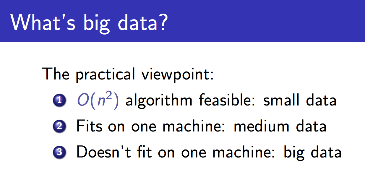
This is John Langford's slide, about what big data is. He says that small data is data for which O(n2) algorithms are feasible. Currently mergic is strictly for this kind of "artisanal" data, where we want to ensure that our matching is correct but want to reduce the amount of human work to ensure that. And we are about to get very O(n2).
Santiago Giraldo,Leonardo Mayer
Santiago Giraldo,Dudi Sela
Santiago Giraldo,Juan Monaco
Santiago Giraldo,S Williams
Santiago Giraldo,C Wozniacki
Santiago Giraldo,S.Giraldo
Santiago Giraldo,Marcos Baghdatis
Santiago Giraldo,Y-H.Lu
...
So we make all possible pairs of identifiers!
One of the things that Open Refine gets right is that it doesn't show us humans all the pairs it's looking at.
All these pairs are annoying for a computer, and awful for humans. The computer can calculate a lot of pairwise distances, but I don't want to look at all the pairs.
Do you see the match here? (It's Santiago again!)
Karolina Pliskova,K PliskovaAside from being a drag to look at, there's a bigger problem with verifying equality on a pairwise basis.
Do these two records refer to the same person? (Tennis fans may see where I'm going with this.)
Kristyna Pliskova,K PliskovaKarolina has a twin sister, and Kristyna also plays professional tennis! This may well not be obvious if you only look at pairs individually. What matters is the set of names that are transitively judged as equal.
sets > pairs
Both perceptually and logically, it's better to think in sets than in a bunch of individual pairs.
workflow support for reproducible deduplication and merging
This is what mergic is for. mergic is a simple tool designed to make it less painful when you need to merge things that don't yet merge.
demo: mergic tennis
With all that background, let's see how mergic attempts to support a good workflow.
$ pew new pydataI'll start by making a new virtual environment using pew.
$ pip install mergicmergic is very new (version 0.0.4.1) and it currently installs with no extra dependencies.
$ mergic -hmergic includes a command-line script based on argparse that uses a default string distance function.
usage: mergic [-h] {calc,make,check,diff,apply,table} ...

positional arguments:
  {calc,make,check,diff,apply,table}
    calc                calculate all partitions of data
    make                make a JSON partition from data
    check               check validity of JSON partition
    diff                diff two JSON partitions
    apply               apply a patch to a JSON partition
    table               make merge table from JSON partition

optional arguments:
  -h, --help            show this help message and exit
In the tennis data, names appear sometimes with full first names and sometimes with only first initials. To get good comparisons, we should:
- Transform all the data to the same format, as nearly as possible.
- Use a good distance on the transformed data.
We can do both of these things with a simple custom script, tennis_mergic.py. It only requires the mergic and python-Levenshtein packages.
#!/usr/bin/env python

import re
import Levenshtein
import mergic


def first_initial_last(name):
    initial = re.match("^[A-Z]", name).group()
    last = re.search("(?<=[ .])[A-Z].+$", name).group()
    return "{}. {}".format(initial, last)


def distance(x, y):
    x = first_initial_last(x)
    y = first_initial_last(y)
    return Levenshtein.distance(x, y)


mergic.Blender(distance).script()
Note that there's a transformation step in there, normalizing the form of the names to have just a first initial and last name. This kind of normalization can be very important.
As a more extreme example, a friend of mine has used the following transform: Google it. Then you can use a distance on the result set to deduplicate.
Now tennis_mergic.py can be used just like the standard mergic script.
$ ./tennis_mergic.py calc names.txt
## num groups, max group, num pairs, cutoff
## ----------------------------------------
##        669,         1,         0, -1
##        358,         5,       384, 0
##        348,         6,       414, 1
##        332,         6,       470, 2
##        262,        85,      5117, 3
##        165,       324,     52611, 4
##         86,       496,    122899, 5
##         46,       584,    170287, 6
##         24,       624,    194407, 7
##         16,       641,    205138, 8
##         10,       650,    210940, 9
##          4,       663,    219459, 10
##          2,       668,    222778, 11
##          1,       669,    223446, 12
There is a clear best cutoff here, as the size of the max group jumps from 6 items to 85 and the number of within-group comparisons jumps from 470 to 5,117. So we create a partition where the Levenshtein distance between names in our standard first initial and last name format is no more than two, and put the result in a file called groups.json:
$ ./tennis_mergic.py make names.txt 2 > groups.jsonThis kind of JSON grouping file could be produced and edited by anything, not just mergic.
As expected, the proposed grouping has combined things over-zealously in some places:
$ head -5 groups.json
## {
##     "Yen-Hsun Lu": [
##         "Di Wu",
##         "Yen-Hsun Lu",
##         "Y-H.Lu",
Manual editing can produce a corrected version of the original grouping, which could be saved as edited.json:
$ head -8 edited.json
## {
##     "Yen-Hsun Lu": [
##         "Yen-Hsun Lu",
##         "Y-H.Lu"
##     ],
##     "Di Wu": [
##         "Di Wu"
##     ],
Parts of the review process would be difficult or impossible for a computer to do accurately.
- There are the Plíšková twins, Karolína and Kristýna. When we see that
K Pliskovaappears, we have to go back and see that this occurred in theUSOpen-women-2013.csvfile, and only Karolína played in the 2013 US Open. - In a similar but less interesting way,
B.Beckerturns out to refer to Benjamin, not Brian. - An
A Wozniakappears withC WozniackandC Wozniacki. The first initial does turn out to differentiate the Canadian from the Dane. - The name
A.Kuznetsovrefers to both Andrey and Alex inWimbledon-men-2013.csv. This can't be resolved bymergic. One way to resolve the issues is to editWimbledon-men-2013.csvso thatA.Kuznetsov,I.SijslingbecomesAlex Kuznetsov,I.Sijsling, based on checking records from that competition. Juan Martin Del Potrois unfortunately too different fromJ.Del Potroin the current formulation to be grouped automatically, but a human reviewer can correct this. Similarly forAnna SchmiedlovaandAnna Karolina Schmiedlova.
After editing, you can check that the new grouping is still valid. At this stage we aren't using anything custom any more, so the default mergic is fine:
$ mergic check edited.json
## 669 items in 354 groups
The mergic diffing tools make it easy to make comparisons that would otherwise be difficult, letting us focus on and save only changes that are human reviewers make rather than whole files.
$ mergic diff groups.json edited.json > diff.jsonNow diff.json only has the entries that represent changes from the original groups.json.
The edited version can be reconstructed from the original and the diff with mergic apply:
$ mergic apply groups.json diff.json > rebuilt.jsonThe order of rebuilt.json may not be identical to the original edited.json, but the diff will be empty, meaning the file is equivalent:
$ mergic diff edited.json rebuilt.json
## {}
Finally, to generate a CSV merge table that you'll be able to use with any other tool:
$ mergic table edited.json > merge.csvNow the file merge.csv has two columns, original and mergic, where original contains all the values that appeared in the original data and mergic contains the deduplicated keys. You can join this on to your original data and go to town.
Here's how we might do that to quickly get a list of who played the most in these 2013 tennis events:
$ join -t, <(sort names.txt) <(sort merge.csv) | cut -d, -f2 | sort | uniq -c | sort -nr | head
##  24 Novak Djokovic
##  22 Rafael Nadal
##  21 Serena Williams
##  21 David Ferrer
##  20 Na Li
##  19 Victoria Azarenka
##  19 Agnieszka Radwanska
##  18 Stanislas Wawrinka
##  17 Tommy Robredo
##  17 Sloane Stephens
Note that this is not the same as the result we got before resolving these name issues:
$ sort names.txt | uniq -c | sort -nr | head
##  21 Rafael Nadal
##  17 Stanislas Wawrinka
##  17 Novak Djokovic
##  17 David Ferrer
##  15 Roger Federer
##  14 Tommy Robredo
##  13 Richard Gasquet
##  11 Victoria Azarenka
##  11 Tomas Berdych
##  11 Serena Williams
As it happens, using a cutoff of 0 and doing no hand editing will still give the correct top ten. In general the desired result and desired level of certainty in its correctness will inform the level of effort that is justified.
distance matters
Having a good distance function might be the most important thing. It's hard to imagine a machine learning as good a distance function as you could just right based on your human intelligence.
There is work on learnable edit distances; notably there's a current Python project to implement hidden alignment conditional random fields for classifying string pairs: pyhacrf. Python dedupe is eager to incorporate this.
See also: Adaptive Duplicate Detection Using Learnable String Similarity Measures
extension to multiple fields
We've been talking about single field deduplication.
name
----
Bob
Rob
Robert
This means that we have one field, say name.
name, name
----------
Bob, Bobby
Bob, Robert
Bobby, Robert
And we look at all the possible pairs and calculate those pairwise distances.

While we described it even in Open Refine as “clustering”, we've really been doing a classification task: either a pair is in the same group or they aren't. We've had one dimension, and we hope that we can just divide true connections from different items with a simple cutoff.
name,    hometown
-----------------
Bob,     New York
Rob,     NYC
Robert,  "NY, NY"
Often, there's more than one field involved, and it might be good to treat all the fields separately.
So let's calculate distances between each field entry for each pair of rows, in this case.
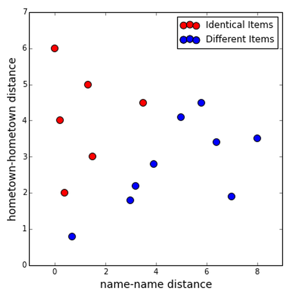
The reason it might be good to treat the fields separately is that they might be more useful together; we might be able to classify all the true duplicates using the information from both fields.
Maybe you can find two clusters, one for true duplicates and one for different items.
Or maybe you could get some training data and use whatever classification algorithm you like.
Let's look at a couple packages that do these things.
R: RecordLinkage
The R RecordLinkage package, which has a good R Journal article and a number of fine vignettes, does quite a lot of interesting things along the lines of what we've been discussing.
You'll also notice that it imports e1071 and rpart and others to plug in machine learning for determining duplicates.
demo: mergic on RecordLinkage data
Let's look at some of the example data that comes with RecordLinkage.
We write the data out to CSV very simply with RLdata500.R:
# install.packages('RecordLinkage')
library('RecordLinkage')
data(RLdata500)
write.table(RLdata500, "RLdata500.txt",
            row.names=FALSE, col.names=FALSE,
            quote=FALSE, sep=",", na="")
Then we can take a look at the data:
$ head -4 RLdata500.txt
## CARSTEN,,MEIER,,1949,7,22
## GERD,,BAUER,,1968,7,27
## ROBERT,,HARTMANN,,1930,4,30
## STEFAN,,WOLFF,,1957,9,2
The data is fabricated name and birth date from a hypothetical German hospital. It has a number of columns, but for mergic we'll just treat the rows of CSV as single strings.
$ mergic calc RLdata500.txt
## ...
##        451,         2,        49, 0.111111111111
##        450,         2,        50, 0.115384615385
##        449,         3,        52, 0.125
## ...
Looking through the possible groupings, we see a cutoff of about 0.12 that will produce 50 groups of two items, which looks promising.
This is slightly artificial, but only slightly so; we could well be doing this for two columns to merge on, in which case so we would hope to find groups of two elements.
$ mergic make RLdata500.txt 0.12
## {
##     "MATTHIAS,,HAAS,,1955,7,8": [
##         "MATTHIAS,,HAAS,,1955,7,8",
##         "MATTHIAS,,HAAS,,1955,8,8"
##     ],
##     "HELGA,ELFRIEDE,BERGER,,1989,1,18": [
##         "HELGA,ELFRIEDE,BERGER,,1989,1,18",
##         "HELGA,ELFRIEDE,BERGER,,1989,1,28"
##     ],
## ...
In this example, the partition at a cutoff of 0.12 happens to be exactly right and we correctly group everything. This says something about how realistic this example data set is, something about your tool of choice if it can't easily get perfect performance on this example data set, and also something about information leakage.
dedupe
The Python dedupe project from DataMade in Chicago is very cool, and I'd better not neglect it.
It's a Python library that implements sophisticated multi-field deduplication and has a lot of connected software. One of these is the csvdedupe.
demo: csvdedupe
We'll use the RecordLinkage data with a header.
write.table(RLdata500, "RLdata500.csv",
            row.names=FALSE,
            quote=FALSE, sep=",", na="")
Then we start the process, specifying which columns of the data to consider for matching.
$ csvdedupe RLdata500.csv --field_names $(head -1 RLdata500.csv | tr ',' ' ')We go into an interactive supervision stage in which dedupe asks us to clarify things. The hope is that it will learn what matters.
You can build this kind of behavior into your own systems; there is an example.
At the end you get output that you can use much like the table output from mergic. It needs some transforming to be easily reviewed by humans though.
real clustering?
The “clustering” that we've been doing hasn't been much like usual clustering.

In part, this is because we we've only had distances between strings without having a real “string space”.
I'm going to just sketch out this direction; I think it's interesting but I haven't seen any real results in it yet.
dog, doge, kitten, kitteh
Say these are the items we're working with. We can use Levenshtein edit distance to make a distance matrix.
       dog doge kitten kitteh
   dog   0    1      6      6
  doge   1    0      5      5
kitten   6    5      0      1
kitteh   6    5      1      0
So here's a distance matrix, and it looks the way we'd expect. But we still don't have coordinates for our words.
Luckily, there is at least one technique for coming up with coordinates when you have a distance matrix. Let's use multidimensional scaling! There's a nice implementation in sklearn.
from sklearn.manifold import MDS
mds = MDS(dissimilarity='precomputed')
coords = mds.fit_transform(distances)
Here's all the code it takes.
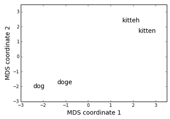
And here's the result! This is at least a fun visualization, and I wonder if doing clustering in a space like this might sometimes lead to better results.
The key thing here is that we're clustering on the elements themselves, rather than indirectly via the pairwise distances.
There are other ways of getting coordinates for words. This includes the very interesting word2vec and related techniques.
Also, you might have items are already naturally coordinates, for example if you have medical data like a person's height or weight.
deep thoughts
By way of conclusion, I'd like to suggest that this problem of deduplication is no good and we should take steps to:
- prevent it from being necessary, by having our systems recommend or enforce standard naming
- make it possible to do deduplication once and reintegrate the results back into the data system
It should be possible to make changes and share them back to data providers. It should be possible to edit data while preserving the data's history. These kind of collaborative data editing are not super easy to implement, and I hope systems emerge that handle it better than current systems.
questions for discussion
I'd like to ask you to consider and discuss with your peers:
- What workflows and tools do you use for these kinds of tasks?
- Does the JSON partition format used by
mergicmake sense for your use? - Does the merge table format used by
mergicmake sense for your use? - What else would make this kind of process better for you?

I also hope to see you at Open Data Science Con in Boston!
Thanks!
Thank you!
@planarrowspace
This is just me again.
I'd love to hear from you!