Visualize co-occurrence graph from document occurrence input using R package 'igraph'

Wednesday January 30, 2013

Co-occurrence can mean two words occurring together in the same document. In this case there are likely to be very many words total, and the following visualization will not necessarily be sensible without judicious data trimming. However there are other cases, for example perhaps the occurrence of two full texts in the same manuscript produced by a scribe in the middle ages, in which the universe of items is reasonably small. In any case where the universe of co-occurring items is fairly small, the following visualization technique might be useful.

For the running example, consider a corpus of three sentences composed of words:

the fat
the cat
the fat fat cat

One step of pre-processing is required: make a table with one column for every element that appears in any collection in the corpus and one row for every collection in the corpus. (It might be done programmatically in some cases, but this will remain outside the current scope.) The values of the table are counts of how many times each element appears in each collection. In some cases this can be a reasonable format even for human-entered data. Load the data into a data frame in R. You probably want to store your data in a separate file, but for convenience we can continue the example:

data <- read.table(header=T, row.names=1, text=
"    the fat cat
 one   1   1   0
 two   1   0   1
 three 1   2   1")

Later we will want to use the number of times each word occurs, so get that now, and prepare to start doing matrix things:

total_occurrences <- colSums(data)
data_matrix <- as.matrix(data)

We want a co-occurrence matrix, which has rows and columns both representing the words (elements) that occur, and the values in the matrix representing the number of times that the elements occur together in the same collection. This is easy to calculate thanks to the nature of matrix multiplication. (You may want to alter the data_matrix by making all entries zero or one, which is easily done with data_matrix <- pmin(data_matrix, 1), because multiple occurrences of the same elements in the same collection lead to multiplicative results; "the the the cat cat" counts as six co-occurrences of "the" with "cat".)

co_occurrence <- t(data_matrix) %*% data_matrix

If you don't have igraph installed, install it. It's as easy as install.packages("igraph"). We'll load it and build our graph object.

library(igraph)
graph <- graph.adjacency(co_occurrence,
                         weighted=TRUE,
                         mode="undirected",
                         diag=FALSE)

That's the extent of the setup! You can start looking around immediately with commands as simple as plot(graph), but you probably want to change some of the display parameters to make the size and color of the visual elements more meaningful, or at least customized. For example, after set.seed(3) for reproducibility:

plot(graph,
     vertex.label=names(data),
     vertex.size=total_occurrences*18,
     edge.width=E(graph)$weight*8)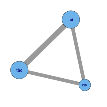

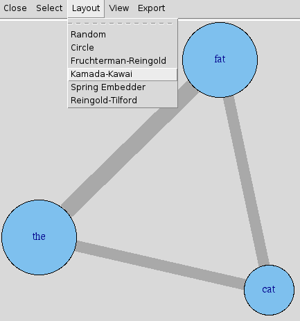
You'll have to experiment with tweaking the option values. You can use mathematical transforms other than just multiplication as well, of course. Other options you may want to add include vertex.color, edge.color, and layout. See R's help for igraph.plotting, but also be sure to play with tkplot in place of plot, which gives you an interactive environment to change things in. It's a good place to try different layouts and just move things around in to explore.

For much more, you can always check out the igraph web site. Their screenshots will quickly give you an overview of what else is possible.

This post was originally hosted elsewhere.